.jpeg)









I've been an M&A advisor for over a decade. I've interviewed over 400 corporate development leaders, private equity operators and integration experts on the M&A Science podcast. One thing that hasn't changed through all these conversations: when serious deal practitioners want to know what a business is really worth, most pull out the same tool: Discounted Cash Flow (DCF) Analysis.
It's not just an M&A phenomenon: research cited by the CFA Institute found that 78.8% of equity analysts use a discounted cash flow approach when valuing individual equities (CFA Institute, citing Pinto, Robinson, Stowe 2019). DCF is the basis for virtually every other valuation technique. And the practitioners I've spoken with who use it effectively are the ones who understand the math and what goes into it.
This guide covers each piece of the DCF model: projecting operating cash flows, estimating terminal value, determining the appropriate discount rate, and stress-testing your assumptions so your output can withstand scrutiny. We'll also discuss where DCF is effective, where it fails, and how it compares to other popular valuation methods. Whether you're valuing a business from scratch or looking to improve an existing model, we aim to give you a working understanding of DCF that goes beyond memorizing the formula.
What Is the Discounted Cash Flow Valuation Model?
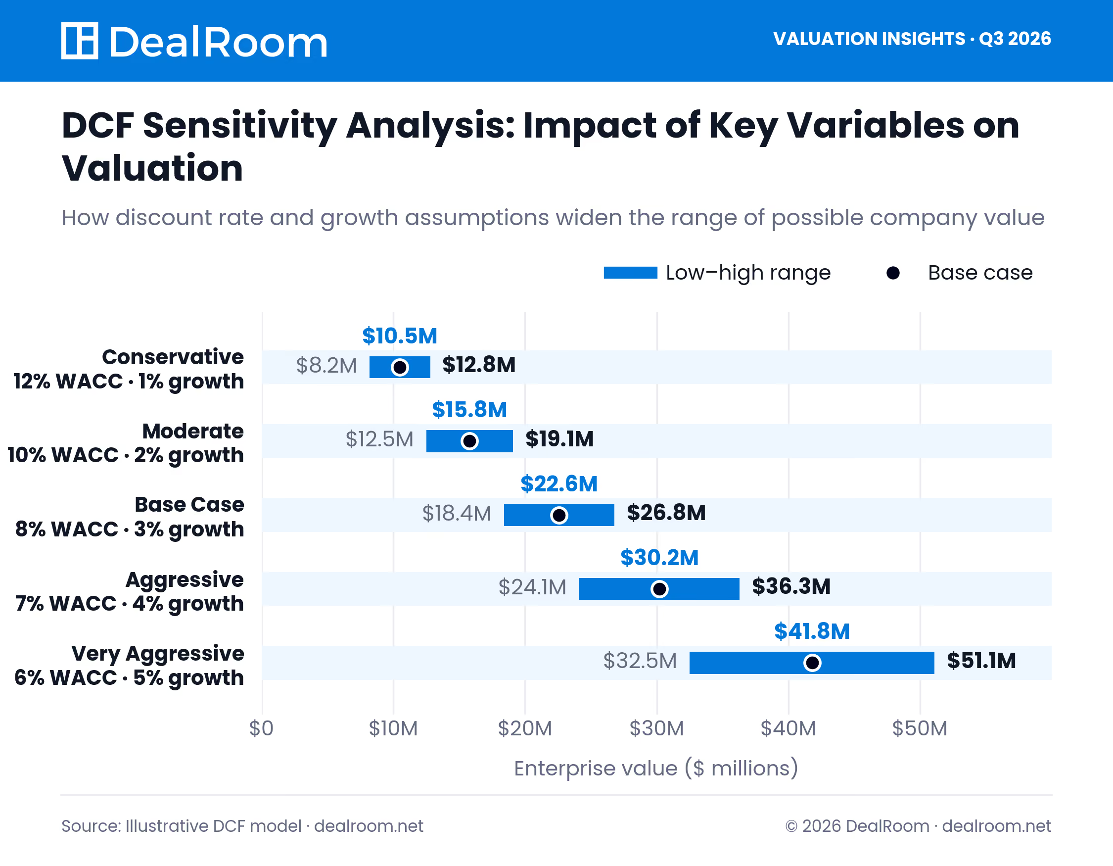
The premise of DCF is simple: a company is worth all of its future cash flows discounted back to their present value. This means projecting how much cash an investment will produce in the future, then calculating what that money would be worth today. Discounted cash flow attempts to quantify that idea. You take all of the future cash flows an investment will produce and discount them back to the present value using a rate that adjusts for risk and the time value of money. The final figure is a calculation of intrinsic value; what the company is really worth on its own merits.
As Harvard Business School Professor Suraj Srinivasan, in the online course Strategic Financial Analysis, explains:
“A DCF analysis is useful when investing money now and expecting some rewards in the future. A DCF analysis finds the intrinsic value of a business, which is the present value of the free cash flow the company is expected to pay its shareholders in the future. If the intrinsic value is higher than the current price, it could be a good investment opportunity.”
What makes DCF so powerful is also what makes it complex and tedious. The output you get is only as good as the assumptions that you feed into the model, and some of those assumptions matter a great deal. Terminal value (the predicted value of a company's cash flows into perpetuity) accounts for roughly three-quarters of the total implied valuation in most DCF models. Sofer Advisors explains:
“Terminal value affects a business appraisal in two direct ways: it drives the majority of total enterprise value in any DCF analysis, and it is the assumption most likely to be challenged by a buyer, IRS examiner, opposing expert, or court.”
Altering the growth rate or discount rate by a few percentage points used to calculate terminal value can swing the projected valuation by millions, if not tens of millions of dollars. According to Sofer Advisors:
“Because terminal value represents 60% to 80% of a DCF’s enterprise value conclusion, even a modest change in the growth rate or exit multiple produces a material shift in the concluded fair market value of the business, with compounding effects on equity value per share in ESOP and 409A contexts.”
That's why understanding how to arrive at each input is as important as memorizing the equation itself.
DCF models are built around projected cash flows. These cash flows can either be free cash flow to firm (FCFF), which is the cash generated by the business before any debt payments, available to both debt and equity holders, or free cash flow to equity (FCFE), the cash remaining for shareholders after all debt obligations have been satisfied. Depending on which cash flow you use, you would use either WACC or cost of equity to discount cash flows back to present value. FCFF is discounted at WACC and FCFE is discounted at cost of equity. Confusing the two is a very common error.
Key Components of the DCF Model
Every DCF contains only three fundamental inputs. Correctly gauging these elements ensures the model functions properly. Estimate them incorrectly and no matter how fancy your spreadsheet looks, the number it gives you will be indefensible.
First, there are the forecasted cash flows. These usually take the form of a five- to ten-year explicit forecast period based on assumptions about revenue growth, operating margins, capital expenditures and changes in working capital.
The second is the discount rate. This represents the cost of capital and the risk characteristics of the business. Typically this is WACC for firm-level valuations and is made up of the weighted cost of equity and after-tax cost of debt.
The third is terminal value, which attempts to account for everything outside of the explicit forecast period. It represents the value of a business that we are assuming will last forever into the future. As such, terminal value essentially lumps decades worth of cash flows into one number, and as mentioned above, it is often the majority of the total valuation. How you calculate it, and the assumptions you make along the way, should be given at least as much scrutiny as the year-by-year projections leading up to it.
Historical Development of DCF
DCF originated with Irving Fisher's 1907 book, The Rate of Interest, and its 1930 sequel, The Theory of Interest, where he explained for the first time that the value of an asset is determined by the present value of its expected future earnings.
DCF originated from the dividend discount model first formalized by John Burr Williams in his 1938 book, The Theory of Investment Value. Williams showed that the intrinsic value of a stock is determined by the discounted present value of its future dividends. Williams' work was expanded on by economist Joel Dean, who in his 1951 book, Capital Budgeting, applied these concepts to capital projects, showing that companies should analyze their capital investments by discounting projected future cash flows. The transition from dividends to free cash flows allowed DCF to evolve from an equity-focused tool to one that focused on free cash flow.
Expanding on Williams' foundational analysis, Myron Gordon and Eli Shapiro published what came to be known as the Gordon Growth Model in 1956. This was the now-familiar constant-growth perpetuity formula still used today to estimate terminal value. During the 1980s and 1990s, DCF became universally accepted in corporate finance and was relied upon with increasing frequency in U.S. courts. DCF has become the preferred valuation method of investment bankers, private equity investors, and corporate financiers.
What's changed since then is less the math itself and more the diligence around it: being more explicit about assumptions, stress-testing terminal value, and employing scenario analysis to portray a range of outcomes rather than one point estimate.
The Basic Principles Behind Discounted Cash Flow Analysis
It can be useful to get a feel for the three concepts underlying a DCF before constructing one yourself. The math is simple once the concepts fall into place. And when a model gives you a number that doesn’t make sense, it’s usually due to one of these being broken somewhere in the assumptions.
The Time Value of Money
One dollar today is worth more than one dollar tomorrow. This isn't merely an accounting trick. Dollars today can be invested at the risk free rate. To receive dollars later is an opportunity cost. The further away the cash flow, the greater the opportunity cost.
That's why we discount. When we discount a future cash flow, we’re essentially asking ourselves: what is this worth to me today, considering both the time I would have to wait to receive it and the risk I would have to endure in order to receive it? The greater the risk/reward trade-off or the longer I have to wait, the more I discount future cash flows, and the lower their value today.
Compounding works both ways. To calculate the future value of money in your pocket today, you compound it forward: FV = PV × (1 + r)^t. To calculate the present value of money you will receive in the future, you discount it back: PV = FV / (1 + r)^t. One constraint: The period of your cash flows and the period of your discount rate must always, always match. Annual cash flows? Annual rate. This is a surprisingly common mistake that silently corrupts your entire model.
Present Value Concepts
Present value is what allows DCF to work. You take your projected cash flow each year of your forecast and discount it back to present value using the formula PV = CF / (1 + r)^t, where t equals how many periods in the future that cash flow occurs. You add up all those discounted numbers (including your discounted terminal value) to get enterprise value.
A few caveats to remember when using it in practice. First, don't average cash flows across years; discount each period's cash flow individually. The time value of money is important, and averaging it out is ignoring that. Second, your forecast period should only be five to ten years. Long enough to see the direction of the business in the near-term future, short enough that your assumptions don't become absurd. Third, you should calculate a terminal value for the business at the end of your projection period instead of letting the model stop. The business will likely still be cash flowing after year 5 or 10, and assuming otherwise will bias you against it. After you have calculated Enterprise Value, subtract net debt and add back any non-operating assets to get Equity Value.
The Discount Rate
The discount rate is by far the most important input into a DCF model. It's also the input for which you have the greatest flexibility in choosing among different methods. Pick the discount rate that most closely aligns with the cash flows you are discounting.
Use WACC if you’re discounting free cash flows to the firm. That is, if the cash flows are before debt payments and are available to provide a return to all capital providers. WACC is calculated as the weighted-average cost of equity and after-tax cost of debt, based on the proportions that the company actually uses to finance its business: WACC = (E / (E + D)) × Re + (D / (E + D)) × Rd × (1 − Tc).
Use the cost of equity if you are discounting free cash flows to equity. That is, if the cash flows are after debt payments and are only available to be returned to shareholders. The cost of equity is most frequently estimated using the Capital Asset Pricing Model (CAPM): Re = Rf + β × (Rm − Rf), where Rf is the risk-free rate of return, β reflects the volatility of the stock relative to the market, and (Rm − Rf) is the equity risk premium. Cost of debt is easier, as it’s simply the effective yield to maturity of the company's debt, reduced by the tax savings due to the interest expense deduction.
Two points of caution. First, never discount different types of cash flows with different discount rates. Discounting FCFF by the cost of equity, or FCFE by WACC will give you a number that doesn't really mean anything because it's internally inconsistent. Second, if the company is changing its capital structure throughout the forecast period, you should update your WACC as needed. If the business is changing its leverage over time (through debt repayment or additional borrowing for example), a discount rate based on today's leverage will not accurately measure the cost of capital five years from now.
If there is extra risk in the business that’s not reflected in your CAPM inputs (illiquidity, early stage risk, concentration risk in one customer or market etc.) increase the discount rate to account for it. What you should never do is alter the cash flows to account for risk. Risk is incorporated in the discount rate, not in an arbitrary discount to the forecast.
Calculating Future Cash Flows
Once the discount rate is determined, the next step is constructing the cash flows it will discount. Essentially this involves forecasting explicit-year cash flows, estimating the terminal value, and ensuring non-cash items don't creep into the forecast.
Projecting Operating Cash Flows
Start with your revenue forecast. Forecast revenue by modeling your assumptions around unit sales, price, and market share.
Turn your revenue forecast into operating profit. Include a clearly defined margin. You should project out gross margin, operating expenses, and tax expenses separately. Operating cash flow = EBIT or NOPAT + depreciation. Subtract capex from operating cash flow.
Forecast working capital. Forecast out accounts receivable, inventory and accounts payable (as days sales outstanding or a percentage-of-sales). Your working capital will have a large impact on your year-end cash balance. Days in working capital will be determined by your operating model.
Free cash flow for the year = NOPAT + depreciation. From here we will subtract capex and change in working capital.
Estimating Terminal Value
You will need to choose whether you want to use the Gordon model or the comparable deals method. If you choose to use the Gordon model, the formula would be:
Terminal Value = FCFn x (1 + g) / (r - g); where g = your long-term growth rate and r = your cost of capital.
Calculate your long-term growth rate g. Remember that this growth rate must be less than your long-term GDP or inflation rate. You must also justify your growth rate based on industry competitive dynamics. If using the comparable deals method, find multiples from comparable deals. Next, multiply to find your stable year EBIT or EBITDA.
Discount the terminal value back to present value using the same discount rate we used to calculate the cash flows. Plug the two methods of calculating terminal value into sensitivity tables to see how they affect valuation.
Eliminate Non-Cash Expenses
Identify any non-cash expenses in your cash flow statements and add them back to the operating profits to arrive at cash available to investors.
Don’t let one-time or non-recurring expenses inflate your typical FCF streams. Normalize the business by using historical cash flow when possible. Consider unique accounting quirks like R&D expenses or leases. Your accounting quirks will need to be translated into cash flow statements.
Determining the Appropriate Discount Rate
Select the discount rate that best represents the actual cost of the business or investment. The discount rate should reflect the cost of capital available to and required by the business or investment.
Weighted Average Cost of Capital
WACC = The weighted average cost of the firm's equity and after-tax debt. WACC is the weighted combination of the firm's cost of equity and cost of debt in proportions to the firm's equity and debt in the market capitalization.
Market capitalization structure is used rather than book capitalization structure because it is what the capital structure looks like at time of calculation.
WACC = (E / (E + D)) * Re + (D / (E + D)) * Rd * (1 - Tc), where E = market equity, D = market debt, Re = cost of equity, Rd = cost of debt, Tc = corporate tax rate.
Keep discount rate and cash flows consistent: Use WACC for unlevered free cash flows and cost of equity for equity cash flows. Update the WACC if the capital structure changes.
Industry-Specific Discount Rates
Different industries command different discount rates depending on the risk profile and capital intensity of each respective industry. Below is a table of discount rates ranges for different industries.
When determining our discount rate, we should always be comparing to the industry of the target firm.
Risk and Return Considerations
When determining the discount rate, we must always match the discount rate with the risks associated with the cash flows. Are the cash flows highly uncertain, long-term, or exposed to highly volatile markets? If so, then we should use a higher discount rate because we can assume greater returns for our investors.
Always separate the risks into systematic and idiosyncratic. When applying the discount rate, we only focus on the systematic risks. Therefore, there will be diversification for idiosyncratic risks.
Always use forward-looking estimates based on current risk-free rate, market risk premium and implied beta.
Cost of Equity vs. Cost of Debt
Cost of Equity (Re): Represents what shareholders would demand. This will always be on the higher side because the shareholder takes more risk when investing in shares. Cost of Equity (Re) can be calculated using the CAPM model, where Re = Rf + beta * (Rm - Rf).
Cost of Debt (Rd): This is the effective yield on new borrowing, which can be estimated from the yields on bonds or debt spreads for similar credit profiles. The after-tax cost will matter more because the interest paid on debt will be tax-deductible, therefore lowering the cost of debt, which will affect WACC.
If your leverage changes at all, you will need to update both Re and Rd. If you increase leverage, you increase Re (because more risk is placed on equity holders) and change the value of Rd (because the spreads will change).
DCF Model Implementation Steps
One, gather historical financial data. Two, define your forecast period and method of calculating terminal value. Three, build your DCF model. In your DCF model you will incorporate your assumptions on revenues, margin, working capital needs, capital expenditures and your discount rate. Make sure your assumptions are accurate and your formulas are consistent. This is where you can eliminate valuation mistakes and keep your DCF model realistic.
Collecting Your Data
When beginning your DCF model, you’ll want to compile three to five years’ worth of audited financial data. This will include the company’s income statements, balance sheets, and cash flow statements. You’ll want to collect line items such as revenues, cost of goods sold, operating expenses, depreciation expense, interest expense, taxes, capital expenditure, and changes in working capital.
Don't ignore non-financial information that may impact your assumptions. Unit volume, price/mix, share, as well as assumptions like GDP, inflation, churn, ARPU, and utilization.
Cross check your sources. SEC filings, company presentations or pitch decks, industry reports, etc. Make sure you trust where your data is coming from. Be cautious of changes in accounting methods or one-time items that may require normalizing. Tidy up your data and build out your model as a time series.
Model Assumptions
An appropriate forecast period must be chosen. Typically, this ranges from 5-10 years. Decide how you will calculate terminal value, either by using the Gordon Growth (perpetuity) method or an exit multiple. Be sure to clearly explain assumptions. Link terminal growth to long-term GDP or industry averages, when possible.
Developing an operating assumption template. Examples would be segment level revenue growth, segment level gross and op margins, EBITDA conversion and how that may change over time. Include working capital days, projected future Capex as a percentage of sales, depreciation schedule, etc.
You want to use the appropriate discount rate based on what types of cash flows you’ll be estimating. If you’re estimating unlevered free cash flow, you should use WACC. If you’re estimating levered free cash flow, you should use cost of debt. You must fully explain all variables and formulas used to come up with this rate. Examples include, but are not limited to Beta, risk free rate, market risk premium, capital structure, etc.
Building the Model
You should have an outline demonstrating how you want your model built. This would involve tabs like Inputs tab, Historical tab, Projections tab, DCF tab, Sensitivity tab. Use formulas to build your model, do not hard code numbers. Life will be much easier for you if your assumptions change.
Have all P&L and cash flow line items be derived from your assumptions. For estimating unlevered free cash flow, calculate it like this: NOPAT = Operating Income * (1-tax rate) + depreciation and amortization - change in net working capital - capital expenditures
Discount these FCFs at your WACC and sum all the discounted cash flows.
Lastly, you want to find the terminal value at the end of your forecast period and discount that too.
Worked Numerical DCF Example
Let's pull all the pieces of a DCF together with an example. Company ABC is a mid-sized software company. Here are our assumptions:
Key Assumptions:
- WACC (Discount Rate): 10%
- Terminal Growth Rate: 2.5%
- Forecast Period: 5 years
Terminal Value Calculation:
At the end of year 5 we calculate our terminal value using the Gordon Growth formula:
- Terminal Value = FCF₅ × (1 + g) / (WACC − g)
- Terminal Value = $14.6M × (1.025) / (0.10 − 0.025)
- Terminal Value = $14.955M / 0.075
- Terminal Value = $199.5M
Present Value of Cash Flows
We discount each year's free cash flow along with the terminal value to present value using the 10% WACC. Below is the full table:
There are two observations from these results. First the math works out nicely, because Company ABC's free cash flows grow at a perfect 10% per year, which results in each year's PV being approximately $9.09M. The real world is not so generous, and growth rates will not be this constant, hence the reason we build our discount table one row at a time.
Second, and more importantly, the terminal value comprises 73% of total Enterprise Value. This is not abnormal. The terminal value usually dwarfs the rest of the DCF. This underscores how small changes in either terminal growth rate or WACC can have huge impacts on enterprise value. A sensitivity table of various combinations of the two should always be included along with this analysis.
To get to equity value, subtract out net debt and add back any non-operating assets to the $169.25M enterprise value number.
DCF vs. Other Valuation Methods
DCF relies on the company’s underlying cash-creating capabilities.
Use DCF when you have high confidence in your long-term cash estimates and want to focus on the intrinsic value of a company. This is best suited for private companies with no public company comparables.
Comparable Companies relies on market-driven valuations of similar companies. Use Comps when you want a market -based sanity-check or are valuing a business similar to public company peers.
Precedent Transactions relies on past M&A transactions. Use Precedent Transactions when you want to get a general sense of control premiums paid in previous M&A deals.
Drawbacks and Issues with DCF
There are several drawbacks and issues with using DCF. The DCF model relies heavily on only a few inputs. You will see wide swings in output results with different inputs.
Sensitivity to Assumptions
The terminal growth rate assumption and discount rate usually have the greatest impact on the value of the DCF. For example, McKinsey research has demonstrated that increasing the cost of capital by just three percentage points for a project with an 8% cost of capital can reduce the project's net present value by between 30% and 40%, depending on the long-term growth rate.
Speculative Forecasts
Trying to predict free cash flows further than three to five years into the future? That's highly speculative. Separate short-term forecasts (based on management's intentions) from long-term assumptions (steady-state operations).
Practical Constraints
Due to complexity of data requirements and modeling, DCF is only relevant in limited scenarios. Startups, and companies with variable cash flows lack the data necessary to forecast a steady-state situation.
Best Practices for Reliable Discounted Cash Flow Valuation
Discounted cash flow modeling is highly detailed. We focus on validation, stress testing and avoiding common modeling errors to produce a clean DCF.
Stress Testing the Model
Stress all inputs to your model. Run your model assuming extreme but realistic assumptions for all inputs. For instance, lower revenue growth for the company by 25% to 50%, lower margins by a few percent, and raise the cost of capital 200-500 points.
Run Multiple Scenarios
Create between three and five scenarios (Base Case, Bear Case, Bull Case, Downside Case, etc.). Using different scenarios will allow you to stress-test variations to key inputs like revenue growth, margins, capital expenditures, and changes to working capital.
Watch Out for Common Mistakes
Avoid assuming any given data point for cost of capital, growth rate, and long-term margins. These variables can have broad ranges and can dramatically swing value. Present a range for each of these variables and leverage market data to justify assumptions around a midpoint.
Ready to put this into practice? Download our free Discounted Cash Flow Valuation Model Excel template to build out your own forecast, terminal value, and discount rate assumptions using a pre-built, formula-driven framework.
Frequently Asked Questions
How do I create a discounted cash flow model in Excel?
Forecast revenue drivers and margins for the duration of your forecast period (typically 5-10 years). Forecast operating line items such as EBIT or NOPAT, changes in working capital, capex, and depreciation to determine free cash flow to firm (FCFF) or free cash flow to equity (FCFE).
Create a discount table and multiply your discount rate by each cash flow. Add the present value of all cash flows plus the terminal value.
What’s the difference between unlevered and levered free cash flows for DCF?
Unlevered free cash flows are cash flows before paying debts (i.e., cash flows that are available for all investors). Levered free cash flows are cash flows after paying debts (i.e., cash flows that are available for equity holders).
How do you choose a discount rate for DCF?
The discount rate for Unlevered DCF is Weighted Average Cost of Capital (WACC). The discount rate for Levered DCF is cost of equity.
Why is the DCF model so sensitive to small changes in inputs?
As terminal value often represents the majority of total enterprise value, minor variations in discount rate or growth rate are amplified. McKinsey research found that increasing cost of capital by three percentage points from 8% reduced present value by 30 to 40%, depending on the assumed long-term growth rate.
What is the difference between calculating terminal value with the perpetuity growth method and exit multiple method?
The Perpetuity Growth Method is calculated using the formula: TV = FCFn x (1 + g)/(r - g). The exit multiple method applies a market derived multiple such as EV/EBITDA or EV/EBIT to a steady state metric in the final forecast year.
How reliable is DCF valuation?
DCF valuation can be very accurate, if the inputs are correct. The accuracy of DCF falls apart at the assumptions; namely, those used to calculate terminal value and the discount rate. Because terminal value makes up 60% to 80% of total enterprise value in a DCF of a going-concern business, small changes to growth rate or discount rate assumptions can have significant impact on the resulting value.
What does DCF valuation offer that other methods do not?
DCF is tied to the underlying business' ability to generate cash, instead of looking at multiples/comps. It’s useful in scenarios where you have an unconventional growth profile or lack of comp data.
What discount rate should I use?
The discount rate should reflect the business risk profile of the investment as well as the capital structure. When you are valuing firms, you should be using the Weighted Average Cost of Capital. When you are valuing shares, you should be using the cost of equity.
Do I use the Gordon Growth model or exit multiple to calculate terminal value?
The Gordon Growth Model and the exit multiple are both used in calculating terminal value. It’s important to note that whenever you pick a method to calculate terminal value, you have to consider whether the business is mature. For mature businesses, you can use the Gordon Growth model to calculate terminal value. If there are comparable companies, then you can use the exit multiple to calculate terminal value. Both of these methods can be used to calculate terminal values in order to see how sensitive your model is.
What is the most common mistake when using DCF model?
The most common mistake while applying the DCF model is over-optimism. When someone is applying the DCF model, they have to be able to defend the numbers used in the calculations. So it's highly recommended to double-check your numbers and run a sensitivity analysis when applying the DCF valuation.









.png)

.avif)


.avif)
.avif)
.avif)

.avif)